TL;DR
- Dense 3D segmentations from sparse 2D annotations, no 3D labels needed.
- 10 minutes of sparse 2D painting bootstraps dense 3D training data.
- Validated across diverse imaging modalities and biological targets.
- Bootstrapped 3D models offer 1000-fold reduction in manual annotation effort.
- Open-source CLI and napari1 plugin, runs on consumer hardware. Scalable to large volumes.
Motivation
Consider a fresh 3D microscopy volume with no annotations. The goal is a dense instance segmentation of some specific structure of interest: cells, organelles, neurites, or other objects. The natural first step is to try existing deep learning models.
Sometimes they work reasonably well, especially when the data resembles what the model was trained on. That is a good sign: it means the model can likely be fine-tuned. But often the data differs enough in imaging modality, tissue type, resolution, or staining that off-the-shelf models produce unusable results.
Segmentation foundation models (SAM2, microSAM3, CellSAM4, Cellpose5, etc.) can help in 2D, but they produce sparse segmentations, lack 3D consistency, and frequently miss the specific structures of interest. The same features that make a dataset scientifically interesting are exactly what generalist models tend to get wrong.
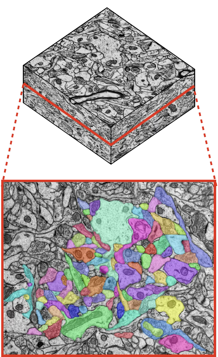
This leads to the same bottleneck every time: manual annotation of objects of interest to generate training data. Dense 3D annotation of even a small volume can take hundreds to thousands of expert hours. For example, dense annotation of hippocampal neuropil in a 180 μm³ EM volume required approximately 2,000 hours of expert effort 6.
We asked: how sparse can the annotations be?
We developed a 2D→3D method that generates dense 3D instance segmentations from sparse 2D annotations. Ten minutes of non-expert painting on a few 2D sections is sufficient to bootstrap 3D segmentations approaching the quality of models trained on dense expert ground-truth on matched evaluation volumes, a 1,000-fold reduction in annotation time. The approach works across diverse imaging modalities, biological targets, and segmentation tasks, and requires no domain-specific pretraining.
Results
Dense 3D segmentations from sparse 2D annotations
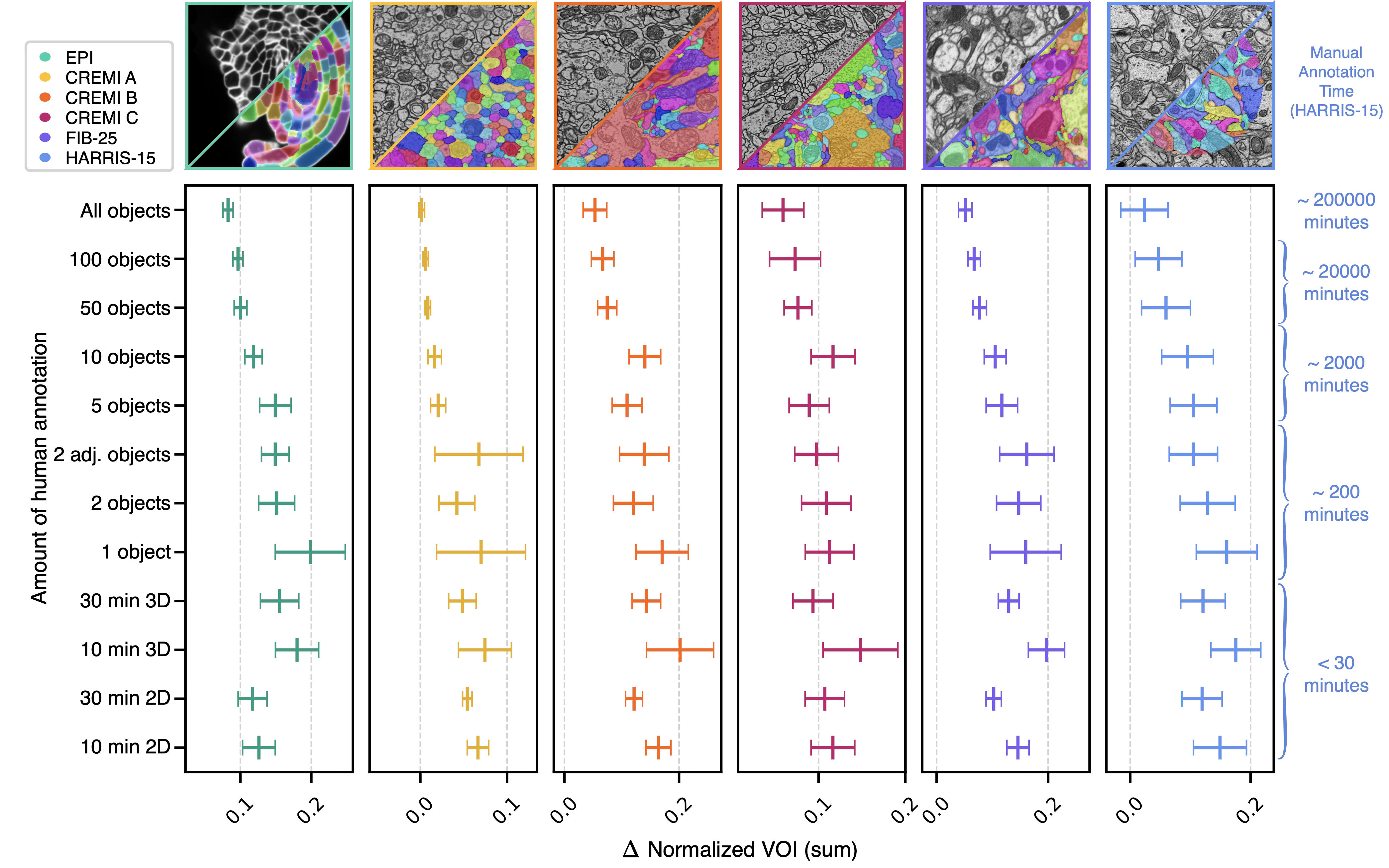
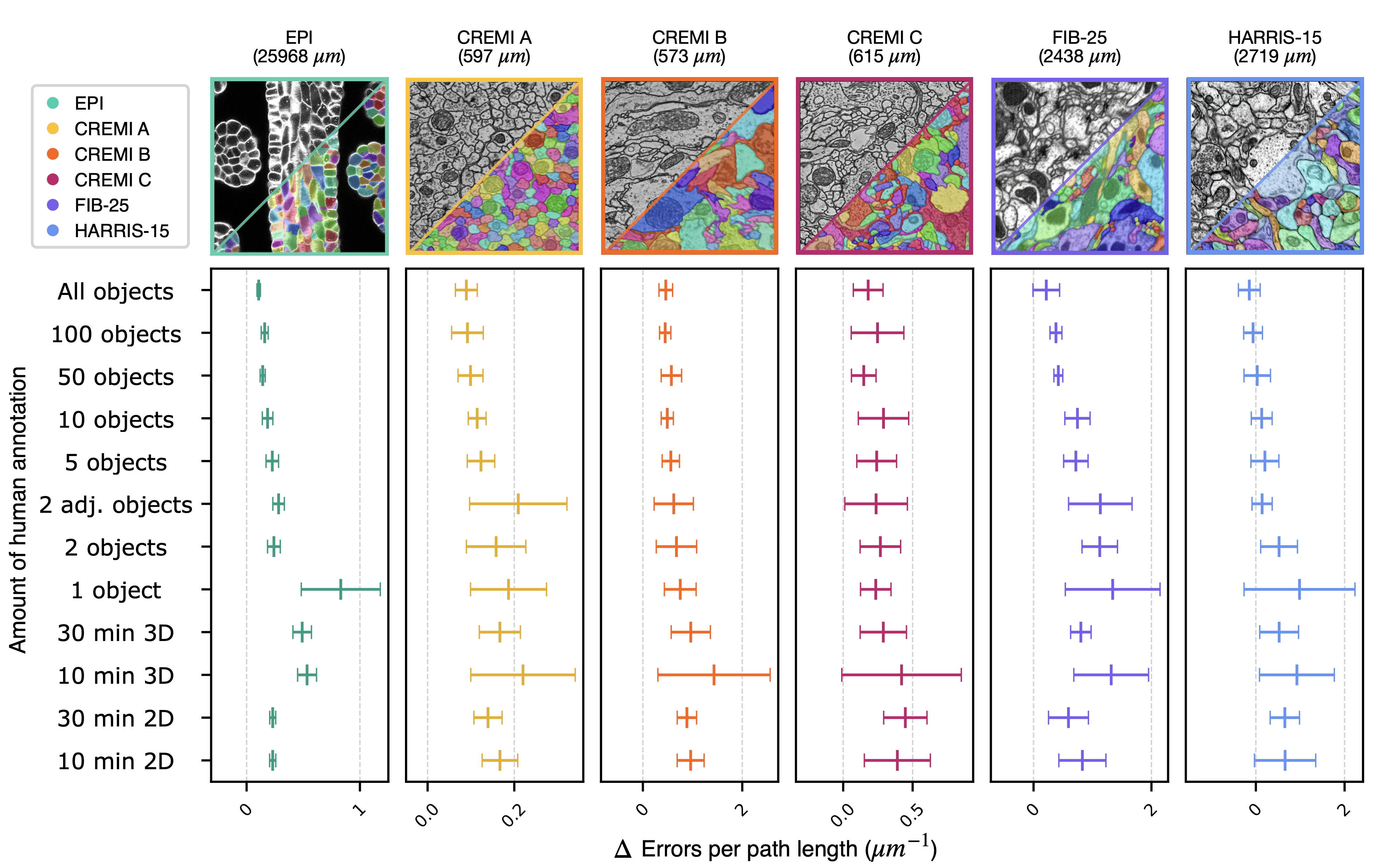
We validated the 2D→3D method across six publicly available datasets: HARRIS-156, FIB-257, CREMI-A/B/C8, and EPI9. Each dataset contains two dense ground-truth volumes. We systematically varied annotation density from single objects to dense labels.
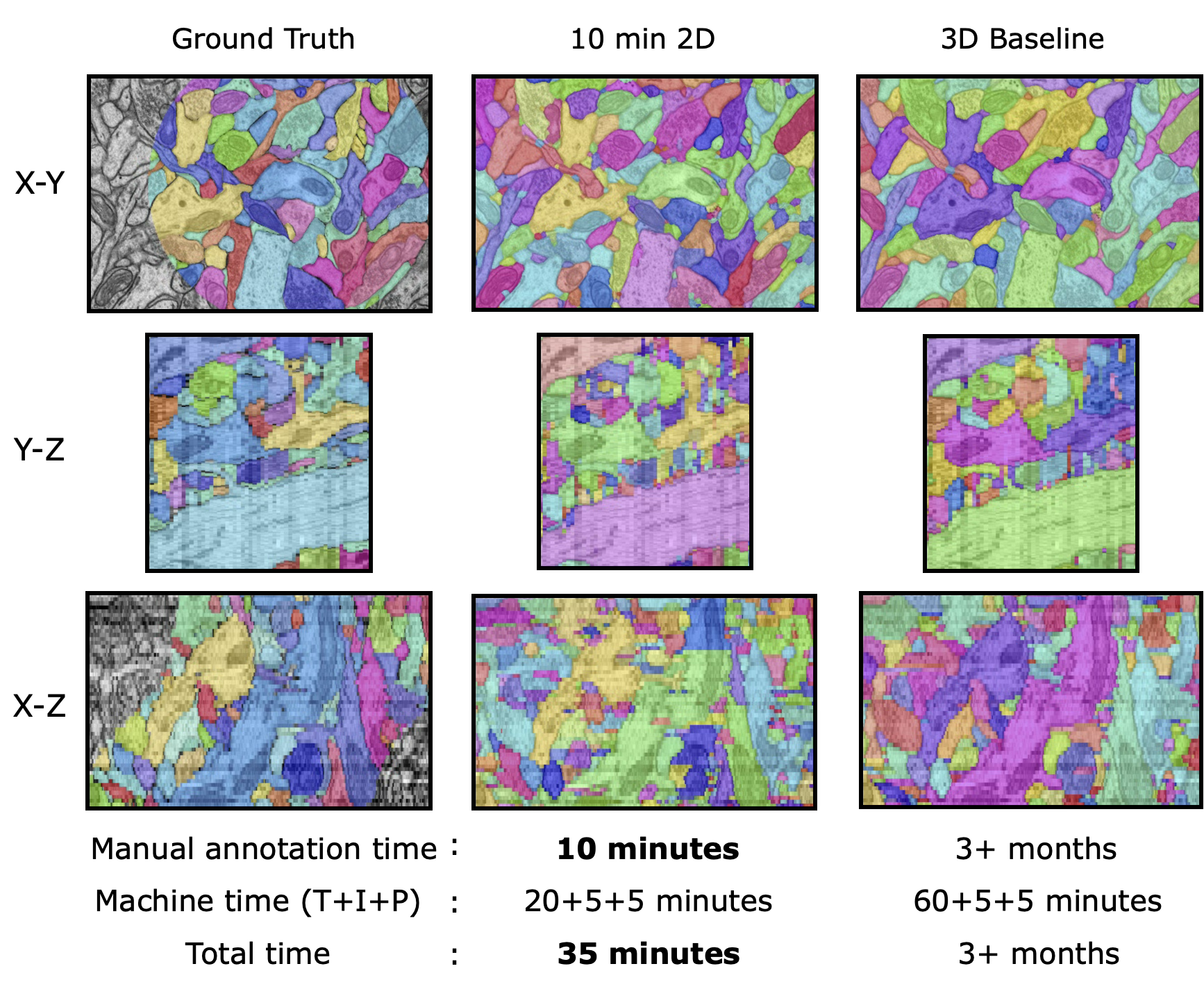
Across all datasets, ten minutes of non-expert sparse annotation on a single section was sufficient to generate a dense 3D segmentation comparable in quality to one based on expert annotation requiring 1,000× more time.
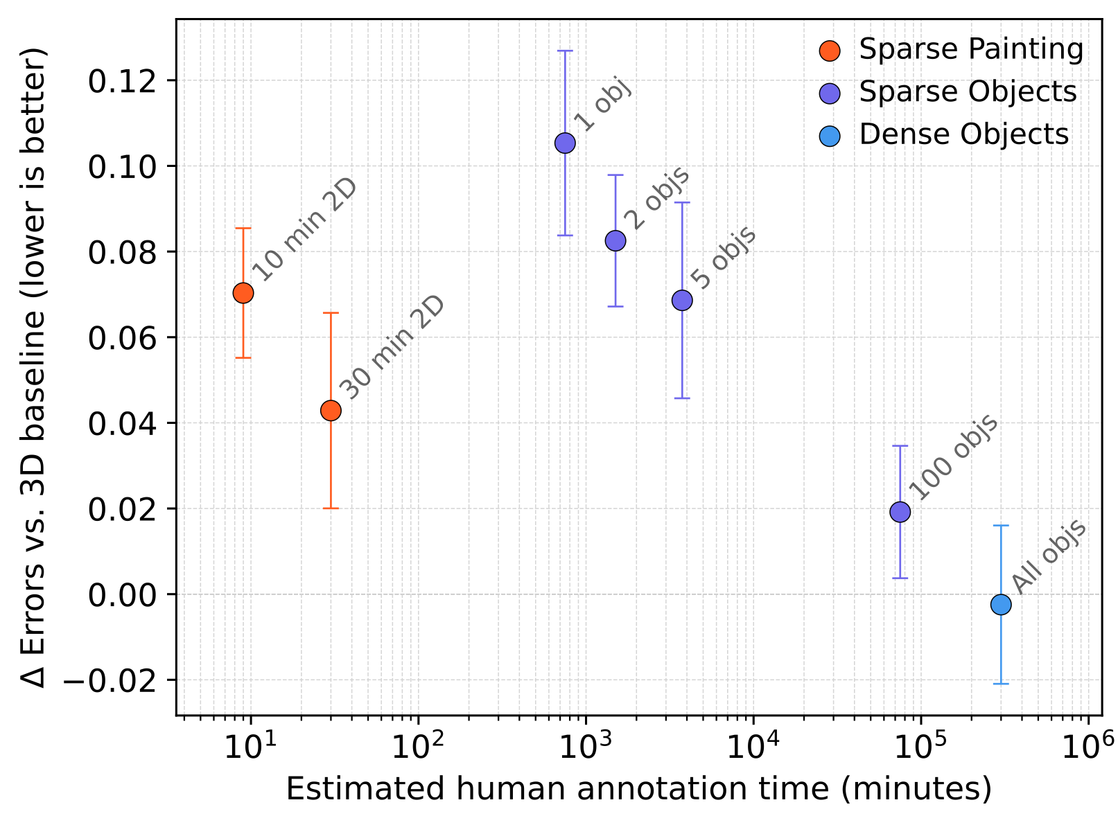
On HARRIS-15, segmentation errors against the dense baseline drop with increasing amounts of annotation, with diminishing returns at each additional order of magnitude of annotation time.
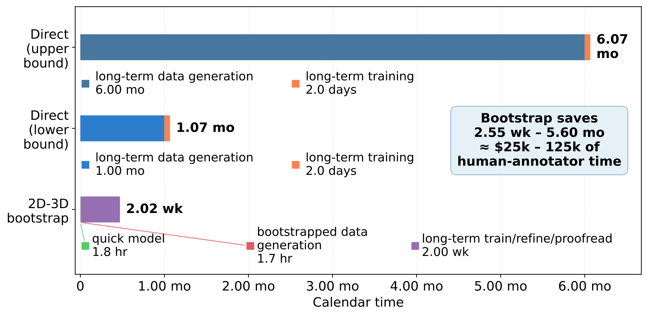
In practical terms, the 2D→3D bootstrap path approaches the quality of direct dense annotation while saving 1-6 months of calendar time and $25k-$125k of expert annotation labor.
Generalization across imaging modalities and segmentation tasks
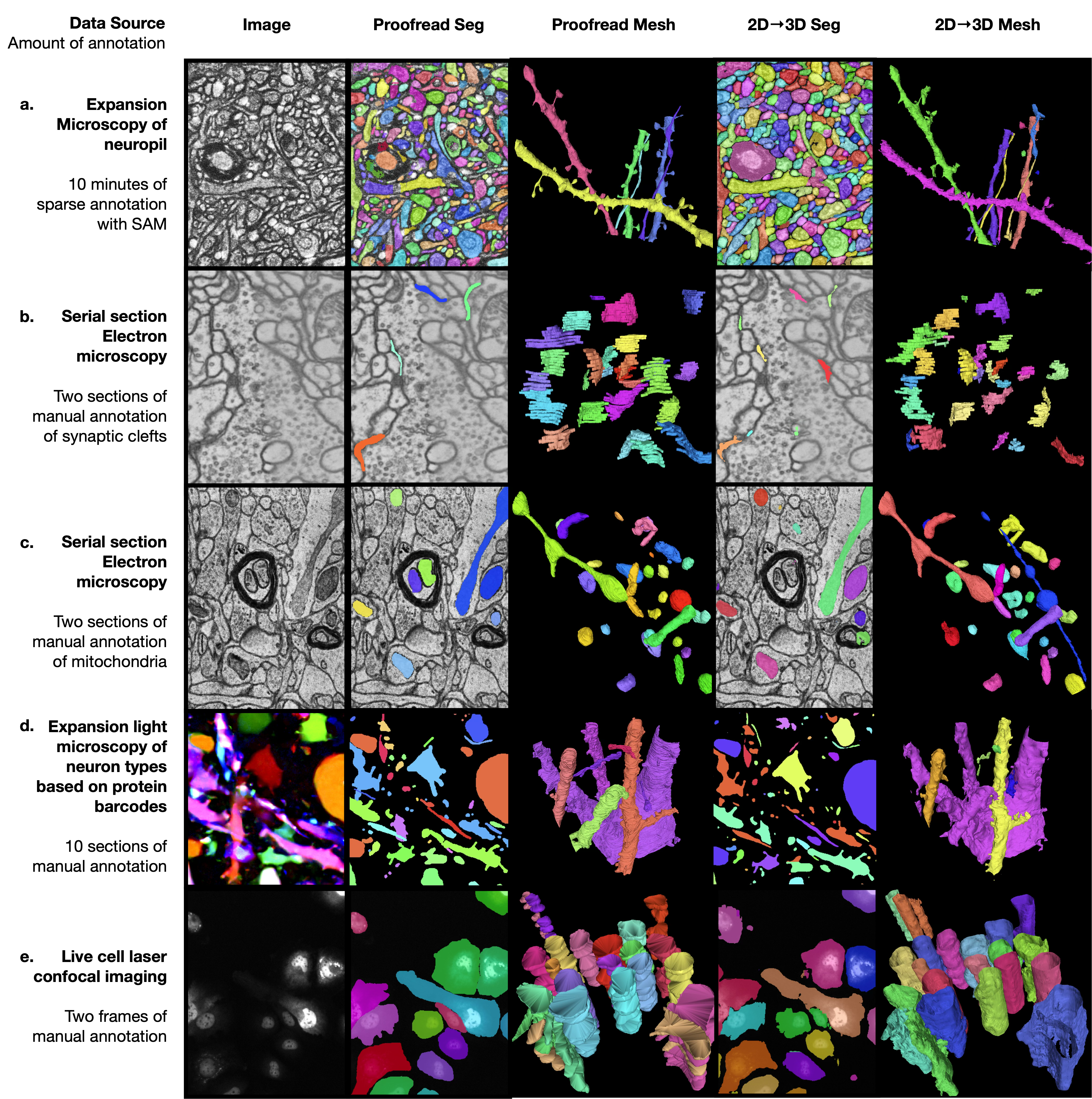
We tested the 2D→3D method on five additional publicly available datasets spanning distinct imaging modalities, biological structures, and segmentation tasks. Across all five, the pipeline produced visually coherent 3D segmentations from minimal annotation effort.
- LICONN10: Expansion-microscopy volumes of mouse somatosensory cortex (effective voxel size ~10 × 10 × 20 nm, x × y × z). 10 minutes of SAM2-assisted sparse annotation on a few sections for boundary segmentation.
- PRISM11: 18-channel light microscopy of mouse hippocampus (voxel size 35 × 35 × 80 nm, x × y × z). Ten sections of manual ground-truth annotation for boundary segmentation.
- CREMI-C8: Serial-section TEM of Drosophila neuropil through an axon tract (voxel size 4 × 4 × 40 nm, x × y × z). Two sections of manual annotation for synaptic cleft segmentation.
- MitoEM-H12: Multi-beam SEM of human cortex (voxel size 8 × 8 × 30 nm, x × y × z). Two sections of manual annotation for mitochondria instance segmentation.
- Fluo-C2DL-Huh713: Live cell laser confocal imaging of Huh7 hepatocarcinoma cells (pixel size 0.65 × 0.65 μm, x × y). Two frames of manual annotation for 2D+t cell segmentation.
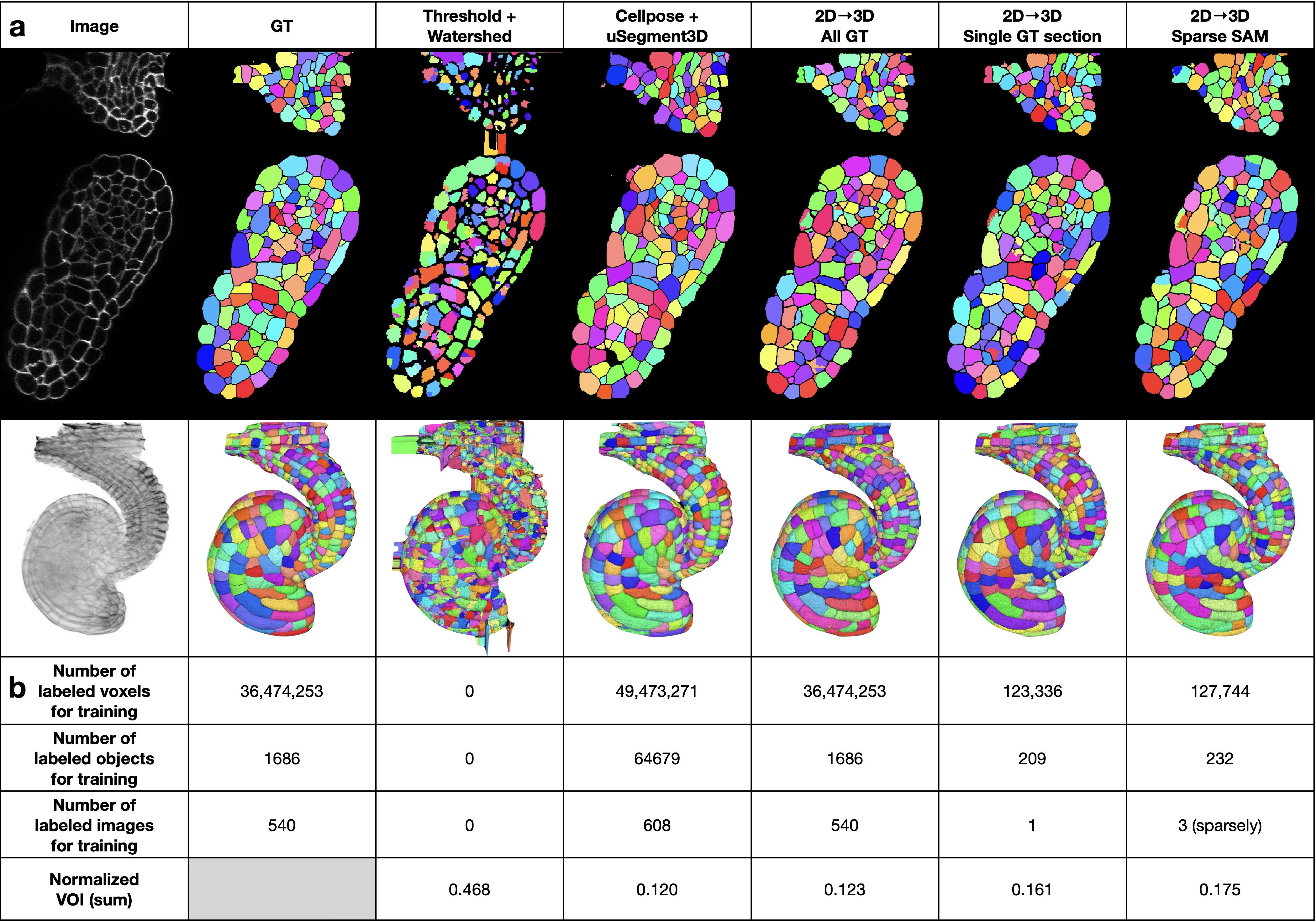
Comparison with existing tools
To contextualize the method against existing general-purpose segmentation tools, we compared it with Cellpose + uSegment3D5,14 on the EPI dataset. Cellpose was applied to all 540 images of the EPI test volume, and uSegment3D was used to merge the 2D segmentations into a 3D consensus segmentation. For the 2D→3D method, we evaluated three levels of supervision: dense ground-truth labels, a single densely labelled section, and sparse SAM-generated labels on 3 images in 5 minutes of human time. The 2D→3D method with sparse SAM labels achieved a usable segmentation from 5 minutes of human effort, approximately two orders of magnitude less annotation for a modest decrease in segmentation accuracy.
Bootstrapping reduces total reconstruction cost
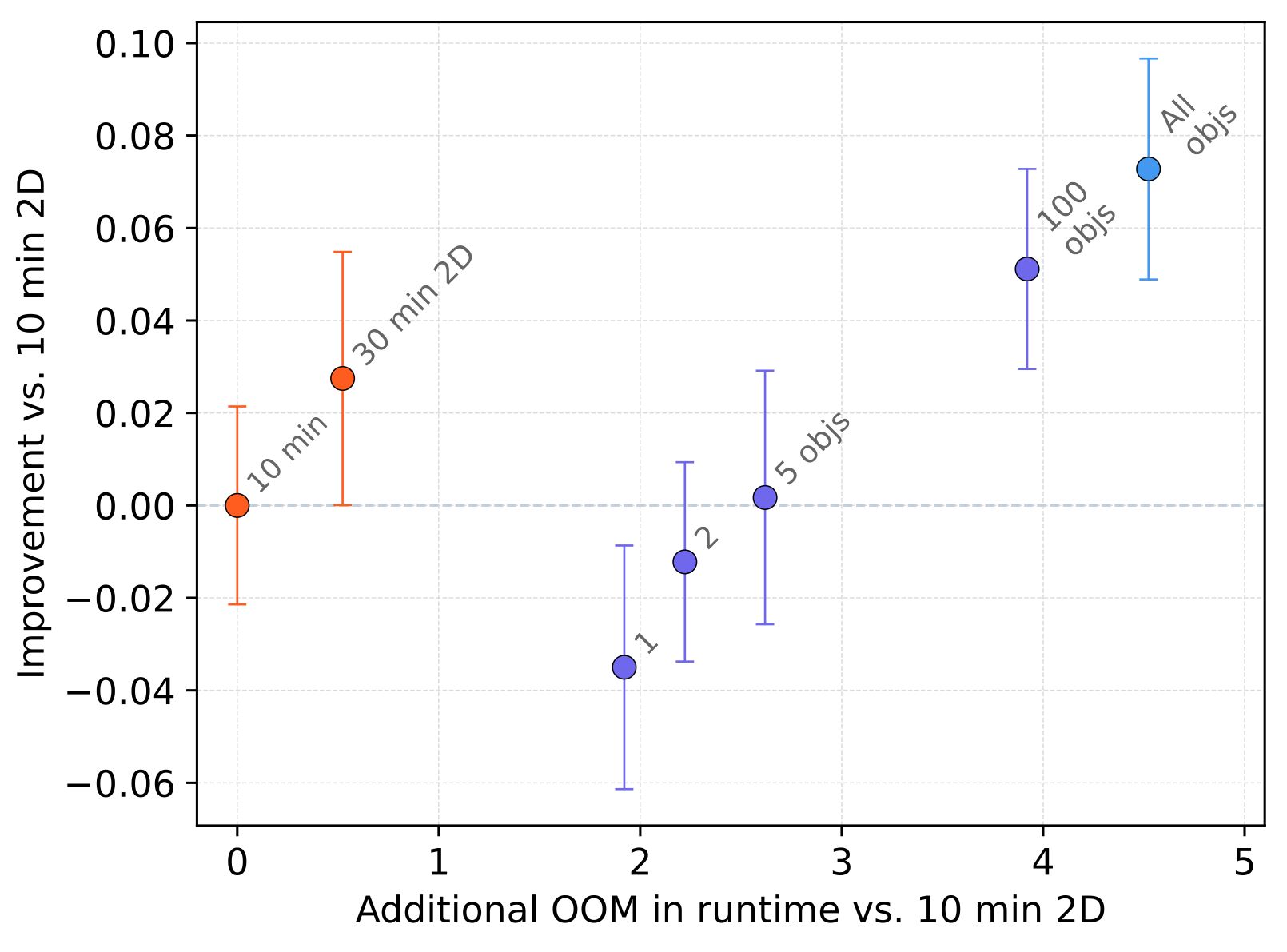
Unproofread 2D→3D segmentations serve as pseudo ground-truth to bootstrap dedicated 3D segmentation models. We evaluated whether segmentations from different amounts of sparse training data could bootstrap subsequent 3D models without any manual proofreading. Across all six datasets, bootstrapped 3D models trained on 2D→3D pseudo ground-truth approached the quality of dense 3D baselines at all sparsity levels.
Pseudo ground-truth from 10 minutes of non-expert annotation on a single section yielded bootstrapped segmentations requiring only approximately 2-3 additional edits per micron (in HARRIS-15) compared to those from dense expert annotations of entire volumes (1,000× more annotation time). Sparser approaches increase the subsequent proofreading burden, but the reduction in upstream annotation yields an order-of-magnitude improvement in total reconstruction time.
Cost-benefit analysis
We estimated the total reconstruction time as the sum of manual annotation time, machine computation time, and estimated proofreading time for HARRIS-15. Proofreading time was estimated at 0.1 minutes per split correction and 1, 3, or 10 minutes per merge correction, spanning the range of reported proofreading throughputs. All times are in Person Workdays (PWD) at 5 hours per day.
| Annotation amount | All objects | 10 objects | 10 min 2D |
|---|---|---|---|
| Total merges to fix false splits | 3,052 | 3,589 | 4,850 |
| Total splits to fix false merges | 1,821 | 2,026 | 2,158 |
| Total edits | 4,964 | 5,723 | 7,156 |
| Time (PWD) | |||
| Manual annotation | 1,000 | 25 | 0.03 |
| Machine computation | 0.3 | 0.3 | 0.3 |
| Proofreading splits (0.1 min/edit) | 0.61 | 0.67 | 1.62 |
| Proofreading merges (1 min/edit) | 7.1 | 7.9 | 8.8 |
| Total (1 min/edit) | 1,008 | 33.9 | 10.7 |
| Proofreading merges (3 min/edit) | 19.2 | 21.5 | 23.2 |
| Total (3 min/edit) | 1,020 | 47.5 | 25.1 |
| Proofreading merges (10 min/edit) | 61.7 | 68.7 | 73.6 |
| Total (10 min/edit) | 1,062.6 | 94.7 | 75.5 |
How It Works
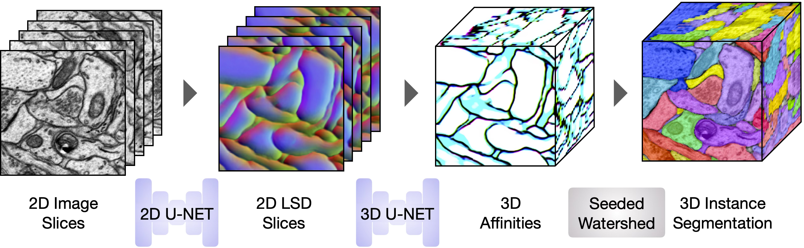
The pipeline operates in two stages. Both use standard U-Net15 architectures and are lightweight enough to run on consumer hardware (<3 GB GPU memory).
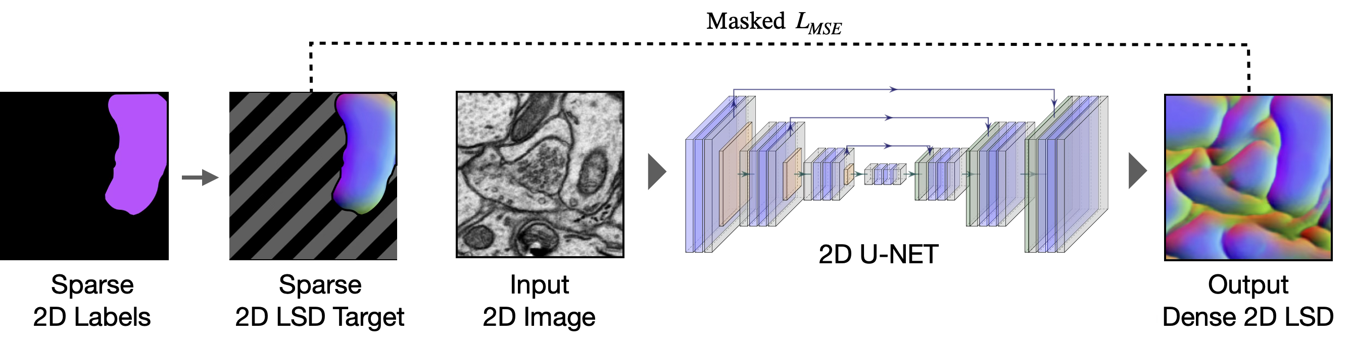
Stage 1: Sparse 2D → Dense 2D
A user creates sparse 2D annotations on one or a few sections, either manually or using a foundation model (e.g., SAM2). A 2D U-Net is trained on these sparse labels to predict dense local shape descriptors (LSDs)16 and affinities17,18. A masked loss restricts supervision to labeled regions, preventing the network from learning background features from unannotated instances. At inference, the 2D network is applied section-by-section to produce a stack of dense 2D predictions.
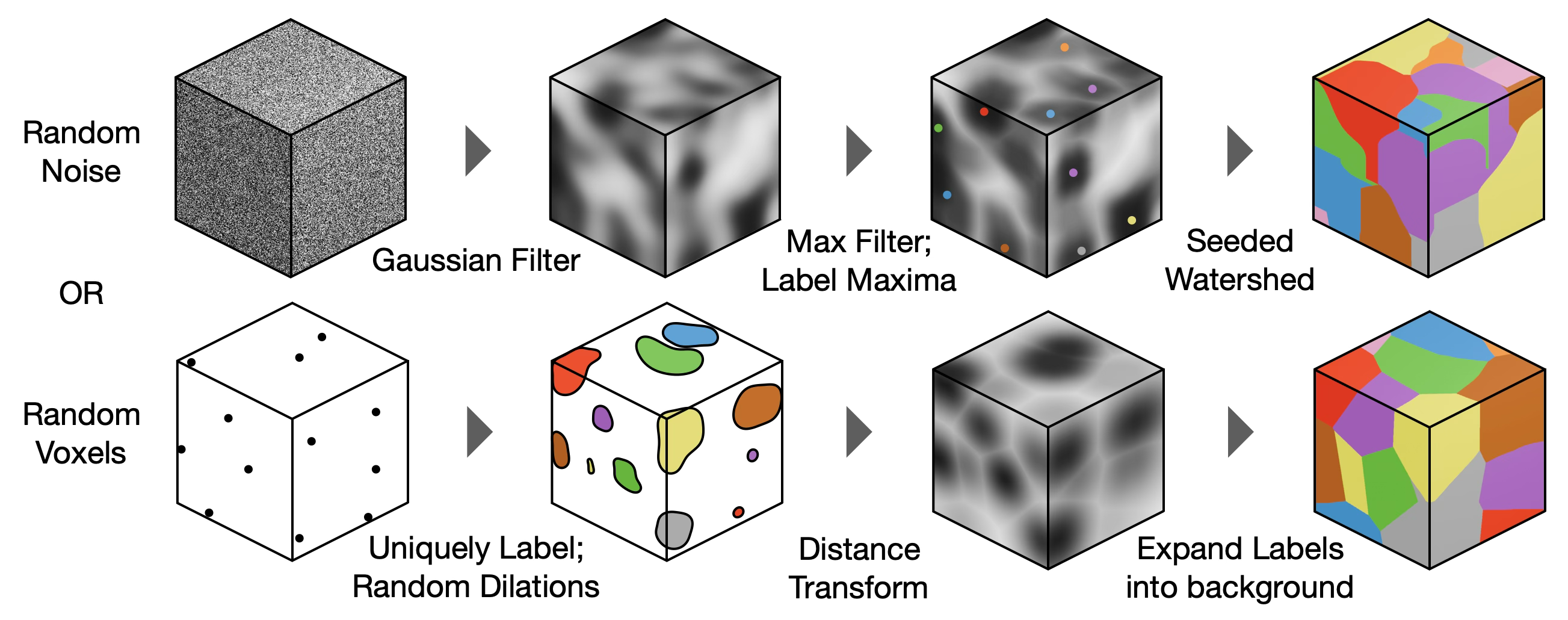
Synthetic 3D Label Generation
Synthetic 3D training data is generated using three distinct strategies to simulate diverse biological structures: morphological dilation from random seeds, section-wise dilation of speckled binary arrays, and watershed on Gaussian-filtered random peaks. A fourth ensemble strategy combines all three equally. These synthetic labels serve as the source of both inputs and targets for the Stage 2 network below and are generated on-the-fly during training.
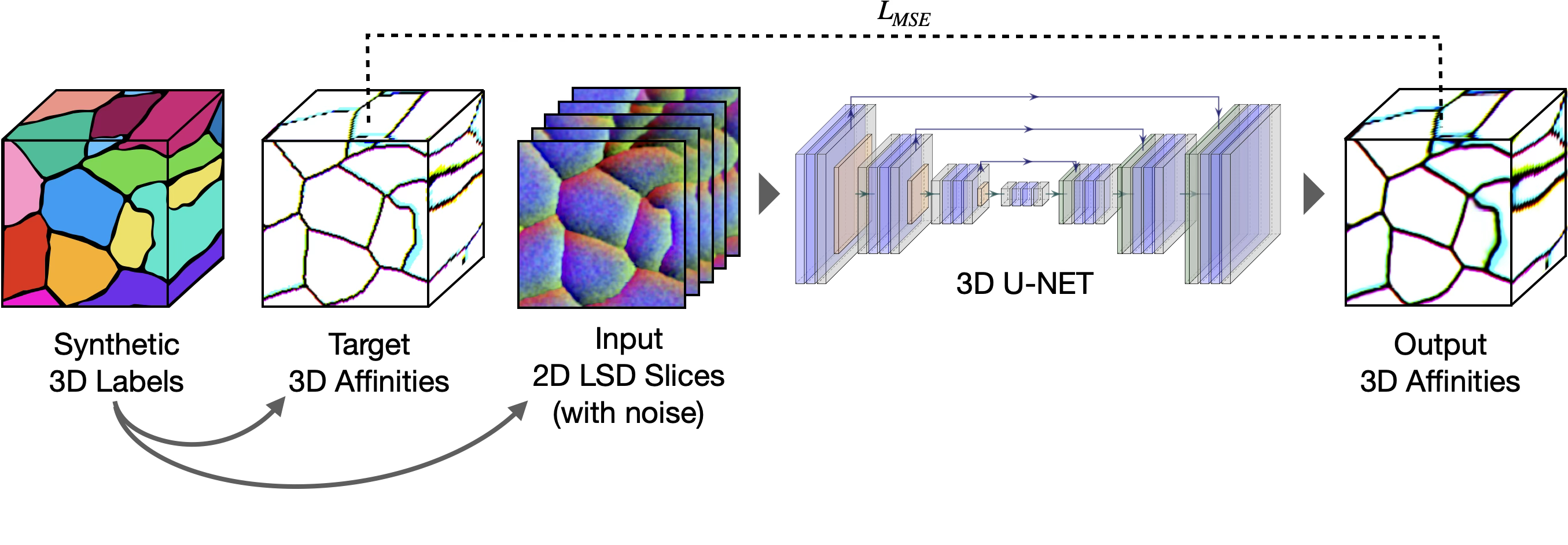
create_labels.py.Stage 2: Stacked 2D → 3D
A lightweight 3D U-Net is pre-trained on the synthetic 3D labels described above. It learns to map noisy stacked 2D LSDs to clean 3D affinities, with both inputs and targets simulated from the synthetic labels. Because the 3D network only ever sees stacked 2D predictions as input, it acquires z-axis connectivity priors entirely from the synthetic data, without requiring any 3D annotation from the target dataset.
Inference
At inference, the two trained U-Nets run sequentially on a target volume. The 2D U-Net is applied section-by-section to produce stacked 2D LSDs, which the 3D U-Net converts to 3D affinities. Seeded watershed on the Stage 2 affinities produces the final 3D instance segmentation.
Get Started
Napari Plugin
The napari-bootstrapper plugin provides an interactive graphical interface for applying the 2D→3D method to small volumes. Create sparse annotations directly in napari, generate dense volumetric segmentations, and perform basic proofreading and post-processing. Works seamlessly with foundation models and the napari plugin ecosystem.
pip install napari-bootstrapper
Bootstrapper CLI
The complete framework is open-source. It includes modules, scripts, and a command line interface for all components of the workflow: data preparation, 2D→3D models, LSD models, training pipelines, blockwise parallel inference and post-processing, evaluation, and error identification. Designed to scale to large volumes using lightweight distributed algorithms that do not require high-performance computing clusters.
pip install bootstrapper
# or
git clone https://github.com/ucsdmanorlab/bootstrapper.git
cd bootstrapper && pip install -e .
Links
- ucsdmanorlab/bootstrapper : Full pipeline (CLI, training, inference, evaluation)
- ucsdmanorlab/napari-bootstrapper : Napari plugin for interactive 2D→3D
- funkelab/gunpowder : Data loading and augmentation
- funkelab/lsd : Local Shape Descriptors
Takeaways
- We present a general-purpose method for generating dense 3D segmentations from sparse 2D annotations. It works across diverse imaging modalities, biological targets, and segmentation tasks. No domain-specific pretraining or high-performance computing is required.
- Specialist 3D models trained on dense ground-truth achieve the highest accuracy within their domain. This method does not replace them. It addresses the bottleneck that precedes them: generating the dense training data needed for both model development and evaluation.
- In our experiments, bootstrapped 3D models trained on unproofread pseudo ground-truth approached the quality of models trained on dense expert annotations, with orders-of-magnitude less human effort.
Complementary to foundation models
The pipeline is complementary to segmentation foundation models. SAM, microSAM, or CellSAM outputs serve directly as sparse input labels for the 2D→3D framework. As 2D foundation models improve, so does every segmentation bootstrapped through them, with no changes to the pipeline itself.
Toward autonomous bootstrapping
The bootstrapper CLI is fully scriptable. AI agents can independently orchestrate the entire bootstrapping loop: selecting annotations, training models, running inference, monitoring LSD and segmentation inconsistencies, and iterating. This paradigm, where agents explore multiple analysis paths in parallel and retain those that meet quality thresholds, could dramatically accelerate ground-truth generation across many volumes simultaneously.
Dense voxel ground-truth remains the gold standard for 3D microscopy segmentation. This method accelerates convergence to that standard by reducing the total cost of generating training data. For laboratories with limited resources, it transforms an intractable annotation problem into a manageable one.
Acknowledgements
U.M. is supported by NIA P30AG068635 (Nathan Shock Center), the David F. and Margaret T. Grohne Family Foundation, Core Grant application NCI CCSG (CA014195), NIDCD R01DC021075-01, NSF NeuroNex Award (2014862), the L.I.F.E. Foundation, and the CZI Imaging Scientist Award from the Chan Zuckerberg Initiative DAF. K.M.H. and V.V.T. are supported by NIH R01MH095980, NSF NeuroNex Technology Hub Award (1707356), NSF NeuroNex Award (2014862), and NSF NCS Award (2219864).
Special thanks to Patrick H. Parker for expert curation and proofreading of the HARRIS-15 dataset, and to all manual annotators. Computing resources provided by the Texas Advanced Computing Center (TACC) at UT Austin.
References
- napari contributors. napari: a multi-dimensional image viewer for Python. Zenodo (2019). doi:10.5281/zenodo.3555620.
- Kirillov, A. et al. Segment Anything. ICCV (2023).
- Archit, A. et al. Segment Anything for Microscopy. Nat. Methods (2025).
- Marks, M., Israel, U., Dilip, R. et al. CellSAM: a foundation model for cell segmentation. Nat. Methods 22, 2585–2593 (2025).
- Stringer, C. et al. Cellpose: a generalist algorithm for cellular segmentation. Nat. Methods 18, 100–106 (2021).
- Harris, K. M. et al. A resource from 3D electron microscopy of hippocampal neuropil for user training and tool development. Sci. Data 2, 150046 (2015).
- Takemura, S. et al. Synaptic circuits and their variations within different columns in the visual system of Drosophila. PNAS 112, 13711–13716 (2015).
- CREMI. cremi.org.
- Wolny, A. et al. Accurate and versatile 3D segmentation of plant tissues at cellular resolution. eLife 9, e57613 (2020).
- Tavakoli, M. R. et al. Light-microscopy-based connectomic reconstruction of mammalian brain tissue. Nature 642, 398–410 (2025).
- Park, S. Y. et al. Combinatorial protein barcodes enable self-correcting neuron tracing. bioRxiv (2025).
- Franco-Barranco, D. et al. Current Progress and Challenges in Large-Scale 3D Mitochondria Instance Segmentation. IEEE Trans. Med. Imaging 42, 3956–3971 (2023).
- Ruggieri, A. et al. Dynamic Oscillation of Translation and Stress Granule Formation Mark the Cellular Response to Virus Infection. Cell Host Microbe 12, 71–85 (2012).
- Zhou, F. Y. et al. Universal consensus 3D segmentation of cells from 2D segmented stacks. Nat. Methods (2025).
- Ronneberger, O., Fischer, P. & Brox, T. U-Net: Convolutional Networks for Biomedical Image Segmentation. MICCAI (2015).
- Sheridan, A. et al. Local shape descriptors for neuron segmentation. Nat. Methods 20, 295–303 (2023).
- Turaga, S. C. et al. Convolutional Networks Can Learn to Generate Affinity Graphs for Image Segmentation. Neural Computation 22, 511–538 (2010).
- Lee, K. et al. Superhuman Accuracy on the SNEMI3D Connectomics Challenge. arXiv:1706.00120 (2017).
Full reference list available in the paper.